"Modern" C++ Lamentations
This will be a long wall of text, and kinda random! My main points are:
- C++ compile times are important,
- Non-optimized build performance is important,
- Cognitive load is important. I don’t expand much on this here, but if a programming language or a library makes me feel stupid, then I’m less likely to use it or like it. C++ does that a lot :)
“Standard Ranges” blog post by Eric Niebler – about C++20 ranges feature – was doing rounds in the game development twitterverse lately, with many expressing something like a “dislike” (mildly said) about the state of modern C++.
I have expressed a similar thought too (link):
That example for Pythagorian Triples using C++20 ranges and other features sounds terrible to me. And yes I get that ranges can be useful, projections can be useful etc. Still, a terrible example! Why would anyone want to code like that?!
Which got slightly out of hand (now 5 days later, that tree of threads is still receiving a lot of replies!).
Now, apologies to Eric for pointing out his post; my lamentation is mostly about “general state of C++” lately. The “bunch of angry gamedevs” on twitter has been picking on Boost.Geometry rationale a year or two ago in a very similar way, and a dozen other times for other aspects of C++ ecosystem.
But you know, twitter not being exactly a nuanced place, etc. etc. So let me expand here!
Pythagorean Triples, C++20 Ranges Style
Here’s the full example from Eric’s post:
// A sample standard C++20 program that prints
// the first N Pythagorean triples.
#include <iostream>
#include <optional>
#include <ranges>   // New header!

using namespace std;

// maybe_view defines a view over zero or one
// objects.
template<Semiregular T>
struct maybe_view : view_interface<maybe_view<T>> {
  maybe_view() = default;
  maybe_view(T t) : data_(std::move(t)) {
  }
  T const *begin() const noexcept {
    return data_ ? &*data_ : nullptr;
  }
  T const *end() const noexcept {
    return data_ ? &*data_ + 1 : nullptr;
  }
private:
  optional<T> data_{};
};

// "for_each" creates a new view by applying a
// transformation to each element in an input
// range, and flattening the resulting range of
// ranges.
// (This uses one syntax for constrained lambdas
// in C++20.)
inline constexpr auto for_each =
  []<Range R,
     Iterator I = iterator_t<R>,
     IndirectUnaryInvocable<I> Fun>(R&& r, Fun fun)
        requires Range<indirect_result_t<Fun, I>> {
      return std::forward<R>(r)
        | view::transform(std::move(fun))
        | view::join;
  };

// "yield_if" takes a bool and a value and
// returns a view of zero or one elements.
inline constexpr auto yield_if =
  []<Semiregular T>(bool b, T x) {
    return b ? maybe_view{std::move(x)}
             : maybe_view<T>{};
  };

int main() {
  // Define an infinite range of all the
  // Pythagorean triples:
  using view::iota;
  auto triples =
    for_each(iota(1), [](int z) {
      return for_each(iota(1, z+1), [=](int x) {
        return for_each(iota(x, z+1), [=](int y) {
          return yield_if(x*x + y*y == z*z,
            make_tuple(x, y, z));
        });
      });
    });

    // Display the first 10 triples
    for(auto triple : triples | view::take(10)) {
      cout << '('
           << get<0>(triple) << ','
           << get<1>(triple) << ','
           << get<2>(triple) << ')' << '\n';
  }
}
Eric’s post comes from his earlier post from a few years back, which was a response to Bartosz Milewski’s post “Getting Lazy with C++”, where a simple C function to print first N Pythagorean Triples was presented:
void printNTriples(int n)
{
    int i = 0;
    for (int z = 1; ; ++z)
        for (int x = 1; x <= z; ++x)
            for (int y = x; y <= z; ++y)
                if (x*x + y*y == z*z) {
                    printf("%d, %d, %d\n", x, y, z);
                    if (++i == n)
                        return;
                }
}
As well as some issues with it were pointed out:
This is fine, as long as you don’t have to modify or reuse this code. But what if, for instance, instead of printing, you wanted to draw the triples as triangles? Or if you wanted to stop as soon as one of the numbers reached 100?
And then lazy evaluation with list comprehensions is presented as the way to solve these issues. It is a way to solve these issues indeed, just that C++ the language does not quite have built-in functionality to do that, like Haskell or other languages have. C++20 will have more built-in things in that regard, similar to how Eric’s post shows. But I’ll get to that later.
Pythagorean Triples, Simple C++ Style
So, let’s get back to the simple (“fine as long you don’t have to modify or reuse”, as Bartosz says) C/C++ style of solving the problem. Here’s a complete program that prints first 100 triples:
// simplest.cpp
#include <time.h>
#include <stdio.h>

int main()
{
    clock_t t0 = clock();

    int i = 0;
    for (int z = 1; ; ++z)
        for (int x = 1; x <= z; ++x)
            for (int y = x; y <= z; ++y)
                if (x*x + y*y == z*z) {
                    printf("(%i,%i,%i)\n", x, y, z);
                    if (++i == 100)
                        goto done;
                }
    done:

    clock_t t1 = clock();
    printf("%ims\n", (int)(t1-t0)*1000/CLOCKS_PER_SEC);
    return 0;
}
We can compile it: clang simplest.cpp -o outsimplest. Compilation takes 0.064 seconds, produces 8480 byte executable, which runs in
2 milliseconds and prints the numbers (machine is 2018 MacBookPro; Core i9 2.9GHz; Xcode 10 clang):
(3,4,5)
(6,8,10)
(5,12,13)
(9,12,15)
(8,15,17)
(12,16,20)
(7,24,25)
(15,20,25)
(10,24,26)
...
(65,156,169)
(119,120,169)
(26,168,170)
But wait! That was a default, non-optimized (“Debug”) build; let’s build an optimized (“Release”) build: clang simplest.cpp -o outsimplest -O2. That takes 0.071s to compile, produces same size (8480b) executable, and runs in 0ms (under the timer precision of clock()).
As Bartosz correctly points out, the algorithm is not “reusable” here, since it’s intermixed with “what to do with the results”. Whether that is a problem or not is outside the scope of this post (personally I think “reusability” or “avoid duplication at all costs” are overrated). Let’s assume it is a problem, and indeed we want “something” that would just return first N triples, without doing anything with them.
What I would probably do, is do the simplest possible thing – make something that can be called, that returns the next triple. It might look something like this:
// simple-reusable.cpp
#include <time.h>
#include <stdio.h>

struct pytriples
{
    pytriples() : x(1), y(1), z(1) {}
    void next()
    {
        do
        {
            if (y <= z)
                ++y;
            else
            {
                if (x <= z)
                    ++x;
                else
                {
                    x = 1;
                    ++z;
                }
                y = x;
            }
        } while (x*x + y*y != z*z);
    }
    int x, y, z;
};

int main()
{
    clock_t t0 = clock();

    pytriples py;
    for (int c = 0; c < 100; ++c)
    {
        py.next();
        printf("(%i,%i,%i)\n", py.x, py.y, py.z);
    }

    clock_t t1 = clock();
    printf("%ims\n", (int)(t1-t0)*1000/CLOCKS_PER_SEC);
    return 0;
}
This compiles and runs in pretty much the same times; Debug executable becomes 168 bytes larger; Release executable same size.
I did make a pytriples struct, where each call to next() advances to the next valid triple; the caller can do whatever it pleases
with the result. Here, I just call it a hundred times, printing the triple each time.
However, while the implementation is functionally equivalent to what the triple-nested for loop was doing in the original
example, indeed it becomes a lot less clear, at least to me. It’s very clear how it does it (some branches and
simple operations on integers), but not immediately clear what it does on a high level.
If C++ had something like a “coroutine” concept, it would be possible to implement the triples generator that would be as clear as the original nested for loops, yet not have any of the “problems” (Jason Meisel points out exactly that in “Ranges, Code Quality, and the Future of C++” post); something like (tentative syntax, as coroutines aren’t part of any C++ standard yet):
generator<std::tuple<int,int,int>> pytriples()
{
    for (int z = 1; ; ++z)
        for (int x = 1; x <= z; ++x)
            for (int y = x; y <= z; ++y)
                if (x*x + y*y == z*z)
                    co_yield std::make_tuple(x, y, z);
}
Back to C++ Ranges
Is the C++20 Ranges style more clear at what it does? From Eric’s post, this is the main part:
auto triples =
    for_each(iota(1), [](int z) {
        return for_each(iota(1, z+1), [=](int x) {
            return for_each(iota(x, z+1), [=](int y) {
                return yield_if(x*x + y*y == z*z,
                    make_tuple(x, y, z));
                });
            });
        });
You could argue either way. I think the “coroutines” approach above is way more clear. C++ way of creating lambdas, and the choice of C++ standard to make things look clever (“what’s an iota? it’s a Greek letter, look how smart I am!”) are both a bit cumbersome. Multiple returns feel unusual if reader is used to imperative programming style, but possibly one could get used to it.
Maybe you could squint your eyes and say that this is an acceptable and nice syntax.
However, I refuse to believe that “us mere mortals” without a PhD in C++ would be able to write the utilities that are needed for the code above to work:
template<Semiregular T>
struct maybe_view : view_interface<maybe_view<T>> {
  maybe_view() = default;
  maybe_view(T t) : data_(std::move(t)) {
  }
  T const *begin() const noexcept {
    return data_ ? &*data_ : nullptr;
  }
  T const *end() const noexcept {
    return data_ ? &*data_ + 1 : nullptr;
  }
private:
  optional<T> data_{};
};
inline constexpr auto for_each =
  []<Range R,
     Iterator I = iterator_t<R>,
     IndirectUnaryInvocable<I> Fun>(R&& r, Fun fun)
        requires Range<indirect_result_t<Fun, I>> {
      return std::forward<R>(r)
        | view::transform(std::move(fun))
        | view::join;
  };
inline constexpr auto yield_if =
  []<Semiregular T>(bool b, T x) {
    return b ? maybe_view{std::move(x)}
             : maybe_view<T>{};
  };
Maybe that is mother tongue to someone, but to me this feels like someone decided that “Perl is clearly too readable, but Brainfuck is too unreadable, let’s aim for somewhere in the middle”. And I’ve been programming mostly in C++ for the past 20 years. Maybe I’m too stupid to get this, okay.
And yes, sure, the maybe_view, for_each, yield_if are all “reusable components” that could be moved into a library;
a point I’ll get to… right now.
Issues with “Everything is a library” C++
There are at least two: 1) compilation time, and 2) non-optimized runtime performance.
Let me allow to show them using this same Pythagorean Triples example, though the issue is true for many other features of C++ that are implemented as part of “libraries”, and not language itself.
Actual C++20 isn’t out yet, so for a quick test I took the current best “ranges” approximation, which is range-v3 (made by Eric Niebler himself), and compiled the canonical “Pythagorean Triples with C++ Ranges” example with it.
// ranges.cpp
#include <time.h>
#include <stdio.h>
#include <range/v3/all.hpp>

using namespace ranges;

int main()
{
    clock_t t0 = clock();

    auto triples = view::for_each(view::ints(1), [](int z) {
        return view::for_each(view::ints(1, z + 1), [=](int x) {
            return view::for_each(view::ints(x, z + 1), [=](int y) {
                return yield_if(x * x + y * y == z * z,
                    std::make_tuple(x, y, z));
            });
        });
    });

    RANGES_FOR(auto triple, triples | view::take(100))
    {
        printf("(%i,%i,%i)\n", std::get<0>(triple), std::get<1>(triple), std::get<2>(triple));
    }

    clock_t t1 = clock();
    printf("%ims\n", (int)(t1-t0)*1000/CLOCKS_PER_SEC);
    return 0;
}
I used a post-0.4.0 version (9232b449e44 on 2018 Dec 22), and compiled the example with
clang ranges.cpp -I. -std=c++17 -lc++ -o outranges. It compiled in 2.92 seconds, executable was
219 kilobytes, and it runs in 300 milliseceonds.
And yes, that’s a non-optimized build. An optimized build (clang ranges.cpp -I. -std=c++17 -lc++ -o outranges -O2)
compiles in 3.02 seconds, executable is 13976 bytes, and runs in 1ms. So the runtime performance is fine, executable
is slightly larger, and compile time issue of course remains.
More on the points above:
Compilation Times Are a Big Issue in C++
Compile time of this really simple example takes 2.85 seconds longer than the “simple C++” version.
Lest you think that “under 3 seconds” is a short time – it’s absolutely not. In 3 seconds, a modern CPU can do a gajillion operations. For example, the time it takes for clang to compile a full actual database engine (SQLite) in Debug build, with all 220 thousand lines of code, is 0.9 seconds on my machine. In which world is it okay to compile a trivial 5-line example three times slower than a full database engine?!
C++ compilation times have been a source of pain in every non-trivial-size codebase I’ve worked on. Don’t believe me? Try building one of the widely available big codebases (any of: Chromium, Clang/LLVM, UE4 etc will do). Among the things I really want out of C++, “solve compile times” is probably #1 on the list, and has been since forever. Yet it feels like the C++ community at large pretends that is not an issue, with each revision of the language putting even more stuff into header files, and even more stuff into templated code that has to live in header files.
To a large extent that is caused by the ancient “just literally paste the file contents” #include model that C++ inherited
from C. But whereas C tends to only have struct declarations and function prototypes in headers, in C++ you often need to put
whole templated classes/functions in there too.
range-v3 is 1.8 megabytes of source code, all in header files! So while the example of “use ranges to output 100 triples” is 30 lines long, after processing header includes the compiler ends up with 102 thousand lines of code to compile. The “simple C++” example, after all preprocessing, is 720 lines of code.
But precompiled headers and/or modules solve this!, I hear you say. Fair enough. Let’s put the ranges header into a
precompiled header (pch.h: #include <range/v3/all.hpp>, include pch.h instead, create the PCH: clang -x c++-header pch.h -I. -std=c++17 -o pch.h.pch, compile using pch: clang ranges.cpp -I. -std=c++17 -lc++ -o outranges -include-pch pch.h.pch). Compilation time
becomes 2.24s, so PCHs do indeed save about 0.7 seconds of compile time here. They do not save the other 2.1s that is longer
than simple C++ approach though :(
Non-Optimized Build Performance is Important
Runtime performance of the “ranges” example is 150 times slower. Two or three times maybe would be acceptable. Anything “over ten times slower”, and it likely means “unusable”. Over hundred times slower? Forget it.
In a real codebase that solves real problems, two orders of magnitude slower likely means that it just would not work on any real data set. I’m working in video games industry; in practical reasons this would mean that Debug builds of the engine or tooling would not work on any real game levels (performance would be nowhere near the needed interactivity level). Maybe there are industries where you run a program on a set of data, and wait for the result, and if it takes 10 or 100 times longer in Debug then it is merely “annoying”. But where something has to be interactive, it turns “annoying” into “unusable” – you literally can not “play” through a game level if it renders at two frames per second.
Yes, an optimized build (-O2 in clang) runs at the same performance as simple C++ version… so “zero cost abstractions”
indeed, as long you don’t care about compilation times, and have an optimizing compiler.
But debugging optimized code is hard! Sure it’s possible, and actually a very useful skill to learn… Similar to how riding a unicycle is both possible, and teaches you an important skill of balance. Some people enjoy it and are really good at it even! But most people would not pick unicycle as their primary means of transportation, similar to how most people don’t debug optimized code if they can avoid it.
Arseny Kapoulkine has a great livestream “Optimizing OBJ loader” where he also ran into “Debug build is too slow” issue, and made it 10x faster by avoiding some of STL bits (commit). As a side effect, it also made compile times faster (source) and debugging easier, since Microsoft’s STL implementation in particular is extremely fond of deeply nested function calls.
That is not to say that “STL is necessarily bad”; it is possible to write an STL implementation that does not become 10x slower in a non-optimized build (as EASTL or libc++ do), but for whatever reason Microsoft’s STL is extremely slow due to over-reliance of “inlining will fix it up”.
As as user of the language, I don’t care whose fault it is though! All I know is that “STL is too slow in Debug”, and I’d rather have that fixed, or I will look into alternatives (e.g. not using STL, re-implementing the bits I need myself, or stop using C++ altogether).
How do other languages compare?
Here’s a brief look at a very similar implementation of “lazily evaluated Pythagorean Triples” in C#. Full C# source code:
using System;
using System.Diagnostics;
using System.Linq;

class Program
{
    public static void Main()
    {
        var timer = Stopwatch.StartNew();
        var triples =
            from z in Enumerable.Range(1, int.MaxValue)
            from x in Enumerable.Range(1, z)
            from y in Enumerable.Range(x, z)
            where x*x+y*y==z*z
            select (x:x, y:y, z:z);
        foreach (var t in triples.Take(100))
        {
            Console.WriteLine($"({t.x},{t.y},{t.z})");
        }
        timer.Stop();
        Console.WriteLine($"{timer.ElapsedMilliseconds}ms");
    }
}
Personally I find the actual bit pretty readable. Compare C#:
var triples =
    from z in Enumerable.Range(1, int.MaxValue)
    from x in Enumerable.Range(1, z)
    from y in Enumerable.Range(x, z)
    where x*x+y*y==z*z
    select (x:x, y:y, z:z);
with C++:
auto triples = view::for_each(view::ints(1), [](int z) {
    return view::for_each(view::ints(1, z + 1), [=](int x) {
        return view::for_each(view::ints(x, z + 1), [=](int y) {
            return yield_if(x * x + y * y == z * z,
                std::make_tuple(x, y, z));
        });
    });
});
I know which one I find cleaner. Do you? Though to be fair, an alternative, “less databasey” form of C# LINQ is pretty busy as well:
var triples = Enumerable.Range(1, int.MaxValue)
    .SelectMany(z => Enumerable.Range(1, z), (z, x) => new {z, x})
    .SelectMany(t => Enumerable.Range(t.x, t.z), (t, y) => new {t, y})
    .Where(t => t.t.x * t.t.x + t.y * t.y == t.t.z * t.t.z)
    .Select(t => (x: t.t.x, y: t.y, z: t.t.z));
How much time it takes to compile this C# code? I’m on a Mac, so I’ll use Mono compiler (which itself is written in C#),
version 5.16. mcs Linq.cs takes 0.20 seconds. In comparison, compiling an equivalent “simple C#” version takes 0.17 seconds.
So this lazy evaluation LINQ style creates additional 0.03 seconds work for the compiler to do. In comparison, the C++ case was creating an additional 3 seconds of work, or 100x more!
This is what you get when “features” are part of the language, as opposed to “it comes as hundred thousand lines of code for the compiler to plow through”.
But can’t you just ignore the parts you don’t like?
Yes, to some extent.
For example here (Unity), we had a joke that “adding Boost into the codebase is a fireable offense”.
I guess that is not true, since sometime last year Boost.Asio
got added, and then I grumbled quite a bit about how it’s super slow to compile, and that merely including <asio.h> includes
whole of <windows.h> with all the macro name hijack horrors that it has.
In general we’re trying to avoid most of STL too. For the containers, we have our own ones, somewhat along the same
reasons as EASTL motivation – more uniform behavior
across platforms/compilers, better performance in non-optimized builds, better integration with our own memory allocators &
allocation tracking. Some other containers, purely for performance reasons (STL unordered_map can’t be fast by design
since the standard requires it to be separately chained; our own hash table uses open addressing instead). Large parts
of the standard library functionality we don’t actually even need.
However.
It takes time to convince each and every new hire (particularly the more junior ones straight from universities) that no, just because it’s called “modern” C++, does not automatically mean it’s better (it might be! or it might be not). Or that no, “C code” does not automatically mean it’s hard to understand, follow or is riddled with bugs (it might be! or it might be not).
Just a couple weeks ago at work I was rambling how I’m trying to understand some piece of (our own) code, and I can’t, since the code is “too complex” for me to get it. Another (junior) programmer drops by, asks me why I look like I’m about to (ノಥ益ಥ)ノ ┻━┻, I say “so I’m trying to understand this code, but it’s way too complex for me”. His immediate response was “ah, old C style code?”, and I was “no, in fact the complete opposite!” (the code I was looking at was some sort of template metaprogramming thingamabob). He hasn’t worked with large codebases, neither C nor C++ yet, but something has already convinced him that “hard to understand” must be C code. I suspect the university; often classes flat out immediately say that “C is bad”, without ever explaining how exactly; but it does leave that impression on the young minds of future programmers.
So yes, I can certainly ignore parts I don’t like about C++. But it’s tiring to educate many others I’m working with, since many are under impression that “modern, must be better” or that “standard library, must be better than anything we could write ourselves”.
Why is C++ this way?
I don’t quite know. Admittedly they do have a very complex problem to solve, which is “how to evolve a language while keeping it close to 100% backwards compatible with many decades of past decisions”. Couple that with that C++ tries to serve many masters, use cases and experience levels, and you do get a complex problem.
But to some extent, it feels like a big part of C++ committee and the ecosystem is focused on “complexity” in terms of showing off or proving their worth.
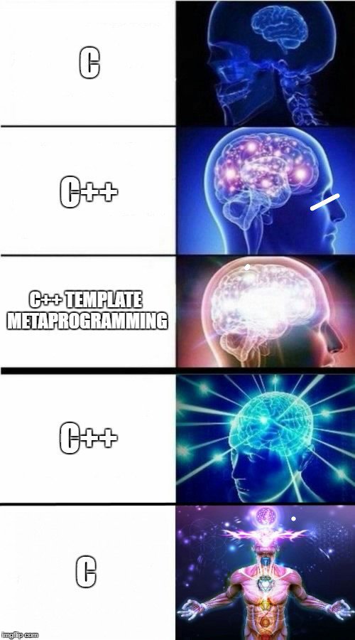
There was this joke on the internet a while ago about typical progression of a C/C++ programmer. I remember myself being in the middle stage, some 16 years ago. Very impressed with Boost, in a sense of “wow you can do that, that’s so cool!”. Without questioning at why you’d want to do that.
Similar to, I don’t know, Formula 1 cars or triple-neck guitars. Impressive? Sure. Marvel of engineering? Of course. Requires massive amount of skill to handle them properly? Yes! Not the right tool for 99% of situations you’d even find yourself in? Yup.
Christer Ericson has put it nicely here:
Goal of programmers is to ship, on time, on budget. It’s not “to produce code.” IMO most modern C++ proponents 1) overassign importance to source code over 2) compile times, debugability, cognitive load for new concepts and extra complexity, project needs, etc. 2 is what matters.
And yes, people who are concerned with state of C++ and the standard libraries can of course join the effort in trying to improve it. Some do. Some are (or think they are) too busy to spend time in committees. Some ignore parts of the standards and make their own parallel libraries (e.g. EASTL). Some think C++ is beyond salvation and try to make their own languages (Jai) or jump ship elsewhere (Rust, subsets of C#).
Taking feedback, and giving feedback
I know how hard it can be, when “a bunch of angry people on the internet” are saying that your work is proverbial dung. I’m working on probably the most popular game engine, with millions of users, and some part of them love to point out, directly or indirectly, how “it sucks”. It’s hard; me and others have put so much thought and work into it, and someone else comes along and says we’re all idiots and our work is crap. Sad!
It probably feels the same for anyone working on C++, STL, or any other widely used technology really. They have worked for years on something, and then a bunch of Angry Internet People come and trash your lovely work.
It’s extremely easy to get defensive about this, and is the most natural reaction. Oftentimes also not the most constructive one though.
Ignoring literal trolls who complain on the internet “just for the lulz”, majority of complaints do have actual issue or problem behind it. It might be worded poorly, or exaggerated, or whoever is complaining did not think about other possible viewpoints, but there is a valid issue behind the complaint anyway.
What I do whenever someone complains about thing I’ve worked on, is try to forget about “me” and “work I did”, and get their point of view. What are they trying to solve, and what problems do they run into? The purpose of any software/library/language is to help their users solve the problems they have. It might be a perfect tool at solving their problem, an “ok I guess that will work” one, or a terribly bad one at that.
- “I’ve worked very hard on this, but yeah sounds like my work is not a good at solving your problem” is a perfectly valid outcome!
- “I’ve worked very hard on this, but did not know/consider your needs, let me see how they can be addressed” is a great outcome too!
- “Sorry I don’t understand your problem” is fine as well!
- “I’ve worked very hard on this, but turns out no one has the problem that my solution is supposed to solve” is a sad outcome, but it also can and does happen.
Some of the “all feedback will be ignored unless it comes in form of a paper presented at a C++ committee meeting” replies that I’ve seen in the past few days sound to me like a not very productive approach. Likewise, defending design of a library with an argument that “it was a popular library in Boost!” misses out on the part of the C++ world that does not think Boost libraries are a good design/solution.
The “games industry” at large, however, is also at fault to some extent. Game technologies are traditionally built with C or C++, just because up until very recently, other viable systems programming languages simply did not exist (now you at least have Rust as a possible contender). For the amount of reliance on C/C++, the industry certainly did not do a good enough job at making themselves visible and working on improving the language, the libraries and the ecosystem.
Yes it’s hard work, and yes complaining on the internet is way easier. And whoever ends up working on future of C++ is not solving “immediate problems” (like shipping a game or whatever); they are working on something much more longer-term. But there are companies who could afford to do this; any of big engine companies or large publishers with central technology groups could totally do it. If that would be worth doing, I don’t know, but indeed it’s a bit hypocritical to say “C++ is nuts and is not what we want”, while never telling the folks who make the language, what it is that “we want”.
My impression is that many in the games technology are “mostly fine” with recent (C++11/14/17) additions to the language itself - lambdas
are useful, constexpr if is great, etc. etc. They tend to largely ignore whatever is getting added into the standard libraries,
both because the design/implementations of STL have issues pointed out above (long compile times, bad Debug build performance), or
are simply not that useful, or the companies have already wrote their own containers/strings/algorithms/… years ago, so why
change something that already works.
Here I say that is enough for a post, I need to get dinner.