Fast blur with animated radius
Almost a year ago, while testing some Blender compositor related things, I noticed that their “Fast Blur” mode is not very fast in some cases, and I started to wonder maybe Blender should get a Dual Kawase blur mode, but that had limitations, and after a whole bunch of poofing around I assembled a bunch of existing blurry ideas into Smol Gaussian.
So! As everyone knows, doing a Gaussian blur in the most naïve way is a cost that grows up as square of the blur radius. But luckily enough, Gaussian is separable, so you can do horizontal & vertical blurs separately, and now the cost scales linearly with radius. That is perfectly fine for blurring just a little bit, but if you need really large blurs, that becomes slow.
There are many ways to make blur scale to larger radii, FrostKiwi has a really good blog post about them: Video Game Blurs (and how the best one works), and the “best one” that the post ends with is Dual Kawase.
Dual Kawase is really simple to implement, runs really fast, and is very nice! Except if you 1) need a smoothly varying blur radius, or 2) need different amounts of horizontal & vertical blur. In my case, I needed both. So I kept on tinkering with trying to extend Dual Kawase, and while I got something that kinda works, I found another way to blur that is much closer to Gaussian shape, and feels nicer when blur radius is animated. Or to phrase it differently, I have discovered what a ton of other people have done as well, which is “downsample, blur, upsample”. There’s quite some details to get through though :)
If your daily reading limit is already up, you can stop here and go check an interactive WebGPU blur playground. Otherwise, continue reading!
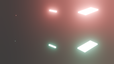
In the videos below, blur radius is animated (increase X&Y together from 5 to 1000, decrease X&Y separately),
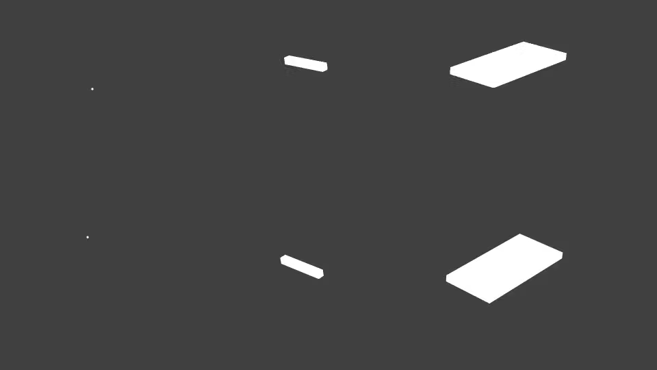
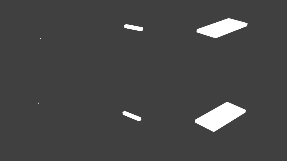
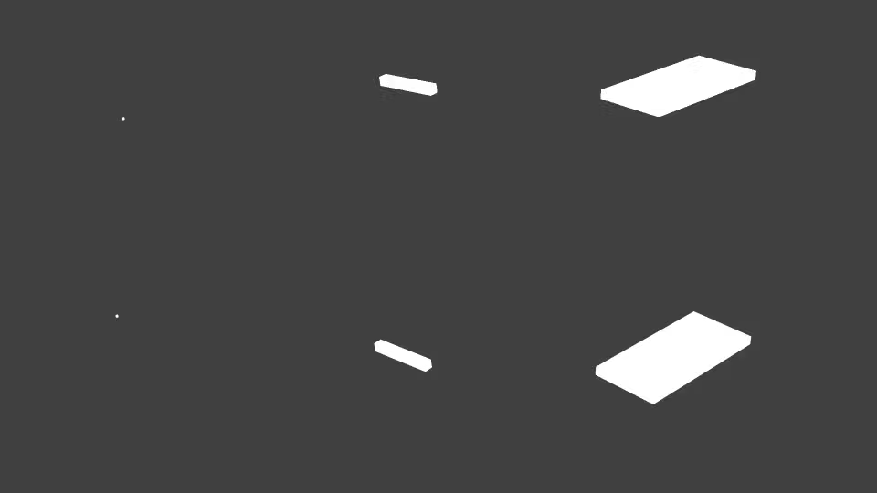
and the input image is rotated during the animation loop. The input image has very bright
objects (linear intensities 500 and 50), here’s the input with additional glare to show “hey I’m bright”
(actual image used for tests has no glare).
Smol Gaussian
Here’s my Smol Gaussian: downsample to a working resolution (which could be different
per axis), apply a small separable Gaussian there, reconstruct to full resolution image.
Here’s how it works in imaginary pseudocode:
Image smol_gaussian(Image input, float2 radius)
{
    float2 sigma = max(radius, 0) / 3;
    int2 orig_size = input.size;
    int2 working_size = orig_size;
    Image image = input;

    // Downsample to the working resolution.
    while (true)
    {
        float2 scale = orig_size / float2(working_size);
        bool2 reduce = (sigma / scale >= 6) && (working_size > 1);
        if (!any(reduce))
            break;
        int2 next_size = select(working_size, ceil(working_size / 2.0), reduce);

        // Integrate source pixel areas, taking care of odd dimensions.
        // Keep one pixel border on reduced axes to preserve input edges.
        // Two consecutive exact halves can be merged into single 4x reduction.
        image = downsample_with_border_preserve(image, next_size);
        working_size = next_size;
    }

    for (axis in {X, Y})
    {
        float scale = float(orig_size[axis]) / working_size[axis];
        float down_variance = (scale * scale - 1) / 12;
        float up_variance = scale == 1 ? 0 : scale * scale *
            (scale > 2 ? 1.0/3 : scale == 2 ? 3.0/16 : 1.0/6);
        // Variance estimates are in original pixels; convert to working pixels.
        float residual_sigma = sqrt(max(0,
            sigma[axis] * sigma[axis] - down_variance - up_variance)) / scale;

        // Regular normalized 1D gaussian pass, extending to 4*sigma, smoothly
        // tapered to zero between 3*sigma and 4*sigma. Pair adjacent weights
        // into bilinear texture samples; skip axes with negligible sigma.
        image = gaussian_pass(image, axis, residual_sigma);
    }

    // Per axis: bilinear up to 2x enlargement, cubic B-spline beyond 2x.
    return reconstruct(image, orig_size);
}
The algorithm is similar to Skia’s GPU Gaussian blur as of 2026 Sep (FilterResult::Builder::blur
and FilterResult::rescale in SkImageFilterTypes.cpp) - independent X/Y scaling, texture samples placed to use
bilinear filtering, one pixel border on downsampled images that preserve the original
image edges (this way bright interiors do not overbright the result at large radius).
Additions compared to Skia blur are:
- When downsampling odd-sized image, we do more correct pixel area integration, so that isolated bright pixels do not flicker with sampling phase shift.
- Downsampled levels are ceil-halved sizes, and downsampling kicks in at sigma=6 (so in practice, blur sizes 18, 36, 72, 144, … switch to new level). Skia instead scales continuously, to keep working sigma under 4.
- When doing the final Gaussian blur, we take into account the blur introduced by downsampling and later reconstruction, i.e. subtract their variance from the blur kernel.
- The final Gaussian kernel extends to sigma=4 (i.e. not truncated at sigma=3), and weights in sigma 3..4 region are tapered to reach zero. This helps to reduce the “blur is cut off” with very bright highlights, and looks better when radius is animated and number of taps changes.
- Final reconstruction to full image size uses a cubic B-spline (fully positive kernel, so no ringing) instead of bilinear, beyond 2x enlargement. This helps to avoid slope discontinuities of bilinear.
- Pairs of exact 2x reductions are done as single 4x reduction as an optimization.
Related work for all of this:
- Skia SkImageFilterTypes.cpp, as mentioned above.
- Fabian Giesen, “Gaussian blur kernels” on gdalgorithms list (2009): low-pass filter, blur at lower resolution, then upsample. He suggests bilinear upsampling is good enough, however in my tests very bright (HDR) blurred objects show bilinear “slope steps”, so I used cubic.
- Intel, “An Investigation of Fast Real-Time GPU-Based Image Blur Algorithms” (2014) has “Working in Lower Resolution” section, but with not much details at when you would switch to it, or how to handle animated blur radius.
- GPU Gems 2, Chapter 20, “Fast Third-Order Texture Filtering” has a trick for cubic B-spline filtering using bilinear samples, which is what I used here in reconstruction part.
All of this is not particularly novel or insightful, I consider it to be perhaps a handful of small quality tweaks compared to Skia blur.
A discarded idea: crossfading working resolutions.
I tried blending neighboring resolutions to hide level switches. Idea was this: when the resolution that does the final blur changes, in theory you could have a visible “jump” if blur radius is animated.
So if resolution switch happens at sigma=6, then starting at sigma=5 already, do both the current resolution and the next resolution, and blend between them using a smoothstep curve. Both evaluations target the same final blur amount, just at different grid, and so each of them uses different amount of gaussian taps.
This however cost performance, since now during transition regions (blur sizes 15..18, 30..36, 70..72 etc.) there are two Gaussian blurs performed and their result is blended. If the X/Y radii are different, we might need to evaluate three Gaussian blurs in fact, and blend between them.
In my testing, this brought pretty much no visual difference, but cost in performance and made the implementation more complex. So eventually this was discarded.
Dual Kawase
The playground also implements an extended version of Dual Kawase. See Marius Bjørge, Bandwidth-Efficient Rendering (SIGGRAPH 2015). The original uses equal horizontal/vertical blur amounts, and only supports a discrete “number of blur pyramid levels” control, not a continuous “blur radius” setting.
For arbitrary blur sizes: blend between neighboring discrete blur levels, similar to
obs-composite-blur.
Blend using the fractional position between steps
remapped with t * (2 + t) / 3, this makes it feel a bit nicer than just a linear blend.
For independent X/Y blur radii: when the smaller blur radius is reached, we stop
further reductions along that axis. For the between-levels blend above, we might need
to blend between three different blurred results.
This works, but does not “feel great” to me. Smoothly animated blur radius does not “feel” smooth on HDR highlights, due to how blending happens between discrete blur levels.
Skia Gaussian
This is what conceptually is closest to “Smol Gaussian”. Implementation in my playground
is just a WebGPU re-implementation of relevant parts of Skia SkImageFilterTypes.cpp, as it
was in revision 15a9437eec87 (2026 Sep). Basic algorithm is:
- Each axis independently downscales to a working sigma
<= 4. Intermediate steps halve the scale, and the last step uses the remaining fractional scale. - A one pixel border around intermediate steps preserves clamped edge colors.
- Final Gaussian pass has radius of
ceil(sigma * 3). A single direct convolution, or separable bilinear-paired filter samples is used depending on size. - Final result is bilinearly upscaled to original resolution.
Skia blur feels just fine on regular LDR content, but on very bright HDR highlights, the aliasing and wobbling are quite apparent.
“Fast Gaussian” (from Blender 5.2)
Blender’s compositor blur node got a “Fast Gaussian” mode back in 2008 (v2.46)
in 2a2453d3,
which however built upon earlier implemented IIR_Gauss functionality for defocus
blur node (2006, v2.43, commit e61dec07).
This builds upon “Recursive Gaussian Filtering”, which if you’re just a programmer but not familiar with signal processing terminology, is quite a confusing name. You’d think a recursive gaussian would be something about building like several smaller versions and somehow combining them, right? Haha nope, not at all, “recursive filter” in signal processing just means that the filter uses some of the previous outputs.
Anyway, the “fast” part is due to filter construction that is basically the same cost, no matter the blur radius. Original code in Blender seemingly was built on one such algorithm, from Young, van Vliet & van Ginkel, “Recursive Gabor Filtering” (2000) paper. Many years later, in 2024 (blender 4.2.0, commit 382131fe) Omar remade this algorithm to have both CPU and GPU code paths, and to avoid double precision. And it was built on a handful of papers, curiously enough an earlier paper by Young, van Vliet et al. “Recursive Gaussian derivative filters” (1998), another paper Deriche “Recursively implementing the Gaussian and its derivatives” (1993), and some more.
Anyhoo, in this project there’s a WebGPU re-implementation of Blender 5.2 “Fast Gaussian” state (mostly recursive_gaussian_blur.cc),
which is fourth order Deriche formulation for radius under 96, and Van Vliet formulation for larger radius.
The algorithms are more or less constant work independent of the blur radius, which is very nice. However, they are also from 25+ years ago, and are not “embarrassingly parallel” that would fit a GPU (or even a many-core CPU) very well. So despite the name, they may or might not be very fast :)
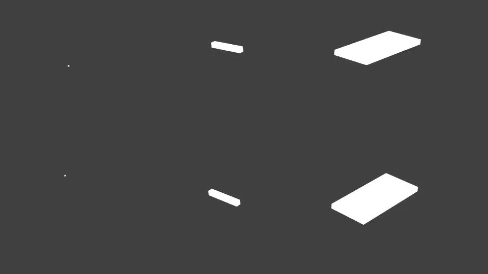
They also have some ringing artifacts, which are not that much noticeable in regular colors, but with very bright HDR highlights,
blurred result can have halos or negative colors, which is not great. See:
“Ryg Blur”
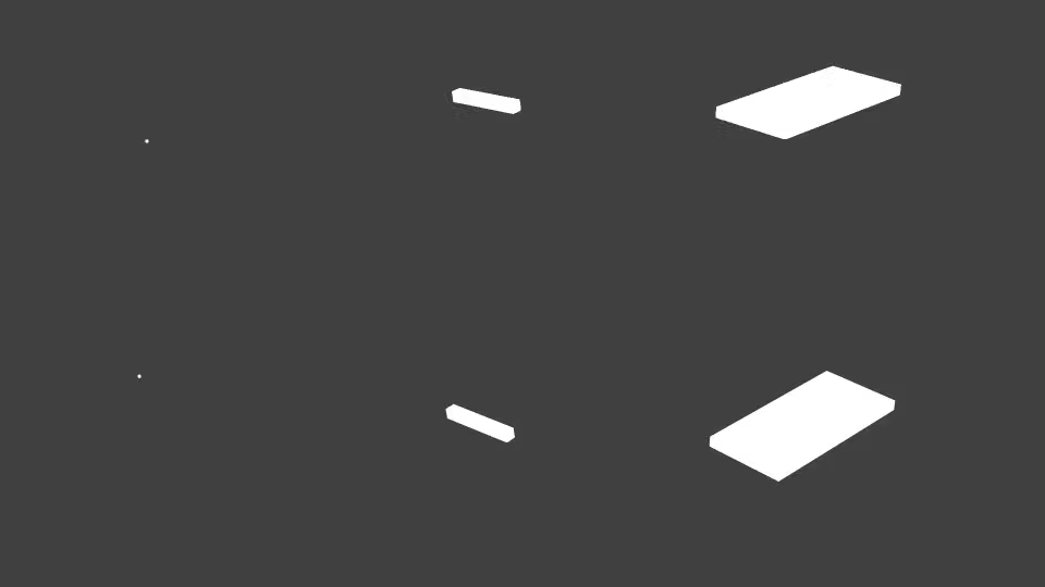
I’m calling this “Ryg Blur” due to Fabian Giesen’s Fast blurs 1 and Fast blurs 2 blog posts (2012), which nicely describe the whole idea, including how exactly to handle fractional samples at the ends, and how trivially that extends to a compute shader implementation.
However the idea itself is “repeated box convolution”, and has been around for ages, e.g. Heckbert “Fun With Gaussians” (1985) talk about it in pages 11-12.
“convolution of a 500x500 image with a 35x35 kernel would take over an hour with 2-D convolution, but only 4 minutes with two 1-D convolutions” where he’s talking about a separable Gaussian filter. Only four minutes to blur a 500x500 image, imagine that! Computers have gotten quite a bit faster, eh.
Anyway, this implementation is basically fixed cost independent of blur size,
and uses two bilinear samples for fractional box endpoint updates. Number of iterations
control is for how many times this box convolution should be done (1: box filter, 2: tent filter,
3 and up: approaching Gaussian). It is very simple to implement, however not the fastest.
Amount of parallelism (parallel over rows or columns) is nowhere near enough to feed modern
GPUs, and multiple passes over the full size image incur a lot of memory traffic.
Regular Gaussian blur
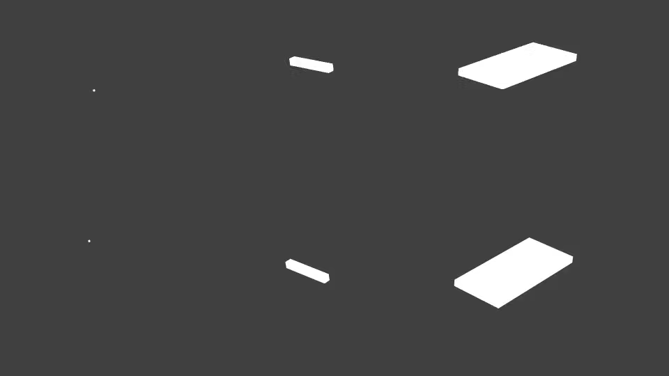
There’s also of course a simple separable Gaussian blur, mostly included as a reference. This is one algorithm that becomes impractical at very large blur radii, since the cost scales linearly with radius. This particular implementation cuts off the kernel at sigma=3 (matches behavior of Blender), which is fine for regular image content, but for very bright HDR highlights it makes the blur feel like it “stops” abruptly. Smol Gaussian feels better in this regard!
Performance
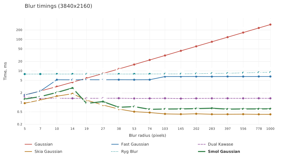
All of the below are in Chrome browser. The timings finish any GPU work, start measuring, do the blur, finish GPU work again, end measuring. So this kinda measures “latency” of doing both CPU & GPU work parts.
Apple M4 Max, macOS:
Ryzen 5950X, RTX 3080Ti, Windows:
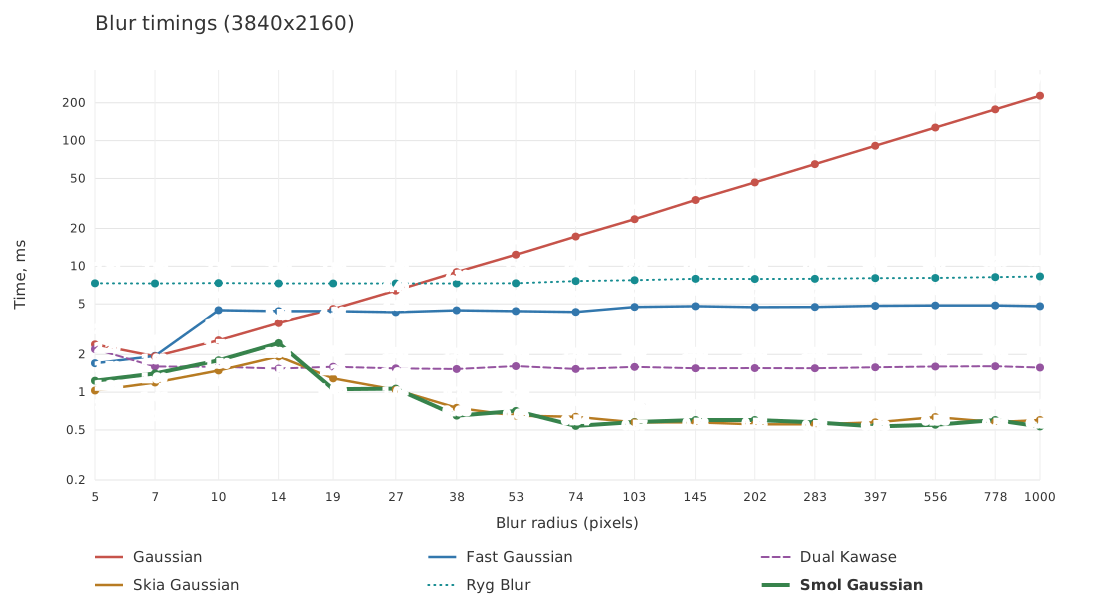
Core i7-1185G7, Intel Iris Xe, Windows:
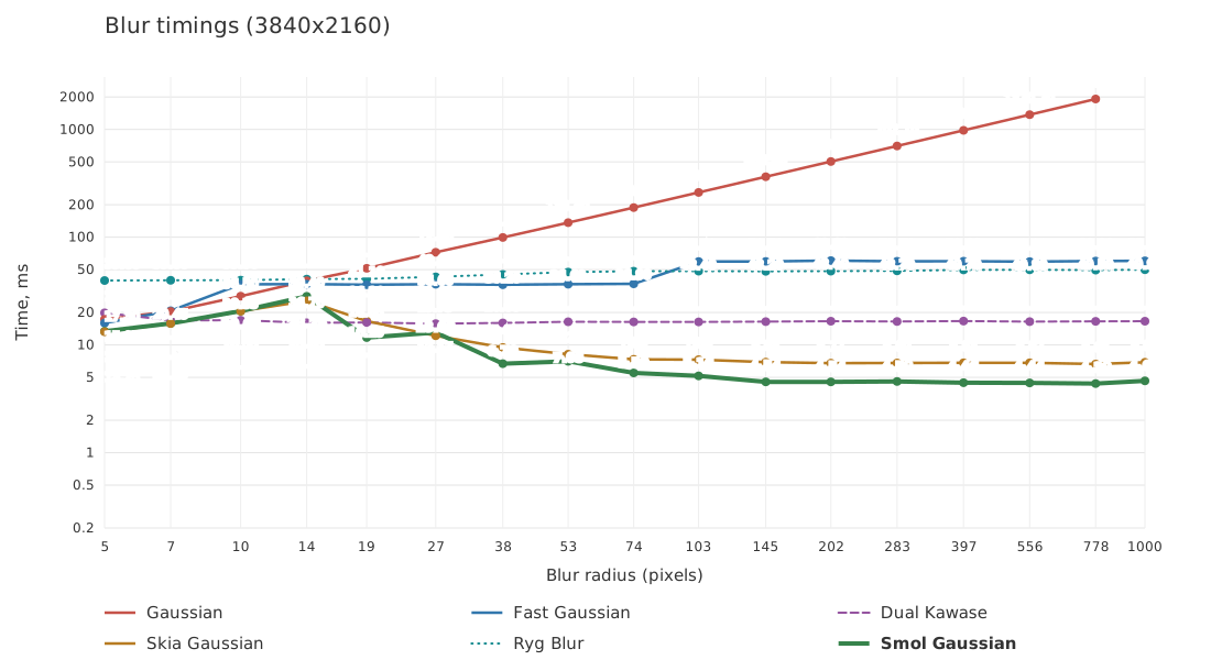
Summary:
- Smol Gaussian is about same performance as Skia blur (same on RTX 3080Ti, a bit slower on M4 Max, a bit faster on Intel Xe). Both of them actually get cheaper as blur radius increases! 🤯 This is because the costly part (actual Gaussian convolution) happens on smaller & smaller image, with the rest being quite cheap.
- Dual Kawase is 2x-3x slower than Smol Gaussian, at least in this implementation that blends between levels and tries to handle non-isotropic blur.
More on the blur playground
Again, there’s an interactive blur playground
and source code for all of it.
Requires WebGPU support (including float32-filterable and float32-blendable).
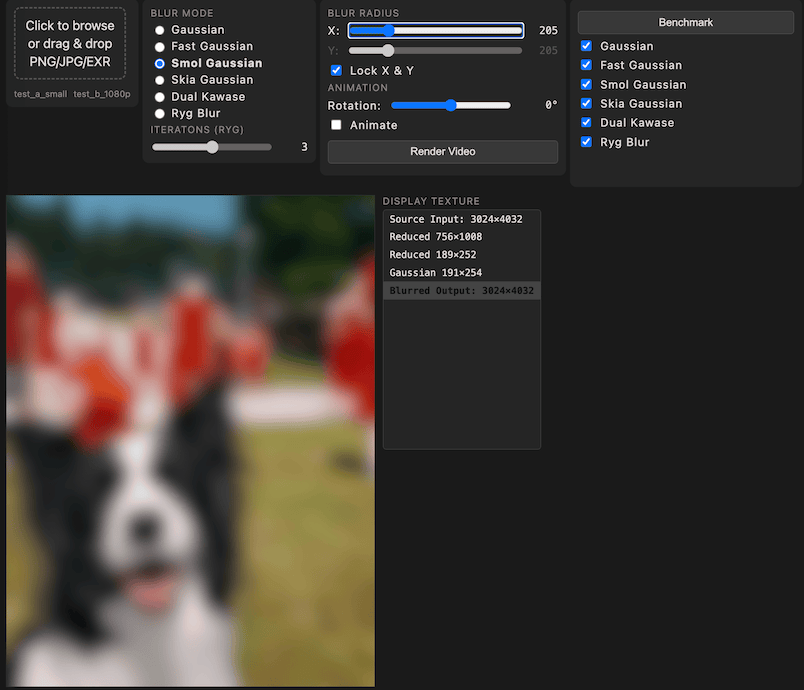
- Pick any of the six blur modes! For free!
- Drag & drop or browse for images (PNG, JPG and a subset of EXR).
test_a_smallandtest_b_1080plinks load two example EXRs. - Adjustable blur radius, with ability to lock X/Y.
- Can inspect various intermediate textures produced by a blurring algorithm.
Animatecheckbox animates the radius and the source image rotation.Render Videobutton exports animated blur result into a video file, using the current blur mode. The video is encoded using WebCodecs browser functionality, and resized to max 960px. Blur itself is performed at full image resolution.Benchmarkbutton tests increasing blur radii with all the selected blur algorithms, and produces a SVG file with the graphs. The result is displayed at the bottom of the page, and can be downloaded too.
Disclosure: I had lollum clankers write javascript & webgpu parts, since I know nothing about this technology. It was both an impressive and quite annoying experience!
Should I try to get this into Blender?
All of this started almost a year ago when I got curious why “Fast Gaussian” does not feel fast in some cases. Well, now I have a WIP pull request with the findings for Blender compositor node (PR 164496). We have not decided what to do with it yet; e.g. should it just replace the existing “Fast Gaussian”, or should it be a new blur mode, or what. That PR also has a CPU implementation (Blender’s compositor today needs to support both GPU and CPU execution), and while some details are different (no paired bilinear sampling on the CPU), it is still several times faster than the current Fast Gaussian, and with no ringing artifacts either.
So, will see how this goes!
Also, if I managed to get something completely wrong about how blurring should work, or there are obvious improvements to do, let me know via email or on mastodon. See ya!