Unity has a problem
From the outside, Unity lately seems to have a problem or two. By “lately”, I mean during the last decade, and by
“a problem or two”, I mean probably over nine thousand problems. Fun! But what are they, how serious they are,
and what can be done about it?
Unity is a “little engine that could”, that started out in the year 2004. Almost everything about games and
related industries was different compared to today (Steam did not exist for 3rd party games! The iPhone was not
invented yet! Neural networks were an interesting but mostly failed tinkering area for some nerds! A “serious”
game engine could easily be like “a million dollars per project” in licensing costs! …and so on). I joined in
early 2006 and left in early 2022, and saw quite an amazing journey within – against all odds, somehow, Unity
turned from the game engine no one has heard about into arguably the most popular game engine.
But it is rare for something to become popular and stay popular. Some of that is a natural “cycle of change”
that happens everywhere, some of that is external factors that are affecting the course of a product, some is
self-inflicted missteps. For some other types of products or technologies, once they become an “industry standard”,
they kinda just stay there, even without seemingly large innovations or a particular love from the user base –
they have become so entrenched and captured so much of the industry that it’s hard to imagine anything else.
Photoshops and Offices of the world come to mind, but even those are not guaranteed to forever stay the leaders.
Anyway! Here’s a bunch of thoughts on Unity as I see them (this is only my opinion that is probably wrong, yadda yadda).
Caveat: personally, I have benefitted immensely from Unity going public. It did break my heart
and make my soul hollow, but financially? Hoo boy, I can’t complain at all. So everything written around here
should be taken with a grain of salt, this is a rich, white, bald, middle aged man talking nonsense.
For better or worse, Unity did take venture capital investment back in 2009. The company and the product was
steadily but slowly growing before that. But it also felt tiny and perhaps “not quite safe” – I don’t remember
the specifics, but it might have very well been that it was always just “one unlucky month” away from running out
of money. Or it could have been wiped out by any of the big giants at the time, with not much more than an
accidental fart in our direction from their side. Microsoft coming up with XNA, Adobe starting to add 3D features
to Flash, Google making O3D browser plugin technology – all of those felt like possible extinction level events.
But miraculously, they were not!
I don’t even remember why and who decided that Unity should pursue venture capital. Might have happened in
one of those “bosses calls” that were about overall strategy and direction that I was a part of, until I wasn’t
but everyone forgot to tell me. I just kept on wondering why we stopped them… turns out we did not! But that’s
a story for another day :)
The first Series A that Unity raised in 2009 ($5.5M), at least to me, felt like it removed the constant worry
of possibly not making it to the next month.
However. VC money is like rocket fuel, and you don’t get rocket fuel just to continue grocery shopping every
day. You have to get to space.
Many clever people have written a lot about whether the venture capital is a good
or a bad model, and I won’t repeat any of that here. It does allow you to go to space, figuratively; but it also
only allows you to go to space. Even if you’d rather keep on going to the
grocery store forever.
A bunch of old-time Unity users (and possibly employees) who reminisce about “oh, Unity used to be different
Back In The Day” have these fond memories of the left side of the graph below. Basically, before the primary
goal of the company became “growth, growth and oh did I mention growth?”.
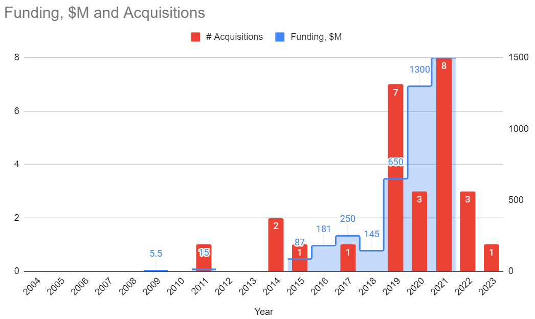
Here’s Unity funding rounds (in millions of $ per year), and Unity acquisitions (in number per year) over
time. It might be off or incomplete (I just gathered data from what’s on the internet, press
releases and public financial reports), but overall I think it paints an approximately correct picture.
Unity had an IPO in 2020 ($1.3B raised as part of that), and in 2021 raised an additional $1.5B via
convertible notes. Also went on a large acquisition spree in 2019-2021.

The “good old Unity” times that some of you fondly remember, i.e. Unity 4.x-5.x era? That’s 2012-2015. Several
years after the initial Series A, but well before the really large funding rounds and acquisitions of 2019+.
The “raising money is essentially free” situation that was a whole decade before 2020 probably fueled a lot of
that spending in pursuit of “growth”.
Vision and Growth
In some ways, being a scrappy underdog is easy – you do have an idea, and you try to make
that a reality. There’s a lot of work, a lot of challenges, a lot of unexpected things coming at you, but
you do have that one idea that you are working towards.
On June 2005 the Unity website had this text describing what all of this is about:
“We create quality technology that allows ourselves and others to be creative in the field of game development.
And we create games to build the insight necessary to create truly useful technology.
We want our technology to be used by creative individuals and groups everywhere to experiment, learn, and create
novel interactive content.
We’re dedicated to providing a coherent and clear user experience. What makes us great is our constant focus on
the clear interplay of features and functionality from your perspective.”
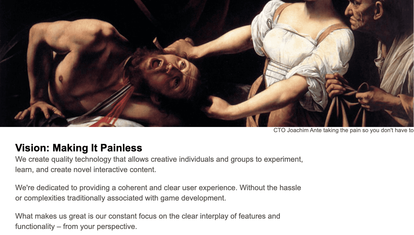
Whereas in 2008, the “about” page was this:

For comparison, right now in 2024 the tagline on the website is this: “We are the world’s leading platform
for creating and operating interactive, real-time 3D (RT3D) content. We empower creators. Across industries
and around the world.” Not bad, but also… it does not mean anything.
And while you do have this vision, and are trying to make it a reality, besides the business and lots-of-work
struggles, things are quite easy. Just follow the vision!
But then, what do you do when said vision becomes reality? To me, it felt like around year 2012 the vision of
“Unity is a flexible engine targeted at small or maybe medium sized teams, to make games on many platforms”
was already true. Mobile gaming market was still somewhat friendly to independent developers, and almost
everyone there was using Unity.
And then Unity faced a mid-life crisis. “Now what? Is this it?”
From a business standpoint, and the fact that there are VCs who would eventually want a return on their
investment, it is not enough to be merely an engine that powers many games done by small studios. So multiple
new directions emerged, some from a business perspective, some from “engine technology” perspective. In no
particular order:
There are way more consumers than there are game developers. Can that somehow be used? Unity Ads
(and several other internal initiatives, most of which failed) is a go at that. I have no idea whether
Unity Ads is a good or bad network, or how it compares with others. But it is a large business branch that
potentially scales with the number of game players.
There was a thought that gathering data in the form of analytics would somehow be usable or monetizable.
“We know how a billion people behave across games!” etc. Most of that thought was before people, platforms
and laws became more serious about privacy, data gathering and user tracking.
Other markets besides gaming. There are obvious ones that might need interactive 3D in some way:
architecture, construction, product visualization, automotive, medical, movies, and yes, military. To be
fair, even without doing anything special, many of those were already using Unity on their own. But
from a business standpoint, there’s a thought “can we get more money from them?” which is entirely
logical. Some of these industries are used to licensing really shoddy software for millions of dollars,
afterall.
Within gaming, chasing “high end” / AAA is very alluring, and something that Unity has been trying
to do since 2015 or so. Unity has been this “little engine”, kinda looked down on by others. It was hard
to hire “famous developers” to work on it. A lot of that changed with JR becoming the CEO. Spending on
R&D increased by a lot, many known and experienced games industry professionals were convinced to join,
and I guess the compensation and/or prospect of rising stock value was good enough too. Suddenly it
felt like everyone was joining Unity (well, the ones who were not joining Epic or Oculus/Facebook at
the time).
Things were very exciting!
Except, growth is always hard. And growing too fast is dangerous.
What is our vision, again?
Unity today is way more capable engine technology wise, compared to Unity a decade ago. The push for
“high end” did deliver way improved graphics capabilities (HDRP), artist tooling (VFX graph, shader
graph, Timeline etc.), performance (DOTS, Burst, job system, internal engine optimizations), and so on.
But also, somehow, the product became much more fractured, more complex and in some ways less
pleasant to use.
Somewhat due to business reasons, Unity tried to do everything. Mobile 2D games? Yes! High end AAA
console games? Yes (pinky promise)! Web games? Sure! People with no experience whatsoever using
the product? Of course! Seasoned industry veterans? Welcome! Small teams? Yes! Large teams? Yes!
At some point (IIRC around 2017-2018) some of the internal thinking became “nothing matters unless it
is DOTS (high-end attempt) or AR (for some reason)”. That was coupled with, again, for some reason,
“all new code should be written in C#” and “all new things should be in packages”. These two led to
drastic slowdowns in iteration time – suddenly there’s way more C# code that has to be re-loaded every
time you do any C# script change, and suddenly there’s way more complex compatibility matrix between
which packages work with what.
The growth of R&D led to vastly different styles and thinking about the product, architecture and
approaches of problem solving. Random examples:
- Many AAA games veterans are great at building AAA games, but not necessarily great at building
a platform. To them, technology is used by one or, at most, a handful of productions. Building
something that is used by millions of people and tens of thousands of projects at once is a
whole new world.
- There was a large faction coming from the web development world, and they wanted to put a ton of
“web-like” technologies into the engine. Maybe make various tools work in the browser as well.
Someone was suggesting rewriting everything in JavaScript, as a way to fix development velocity,
and my fear is that they were not joking.
- A group of brilliant, top-talent engineers seemed to want to build technology that is the
opposite of what Unity is or has been. In their ideal world, everyone would be writing all the
code in SIMD assembly and lockless algorithms.
- There was a faction of Unity old-timers going “What are all these new ideas? Why are we doing them?”.
Sometimes raising good questions, sometimes resisting change just because. Yes, I’ve been both :)
All in all, to me it felt like after Unity has arguably achieved “we are the engine of choice for almost
every small game developer, due to ease of use, flexibility and platform reach”, the question on what
to do next coupled with business aspects made the engine go into all directions at once. Unity stopped
having, err, “unity” with itself.
Yes, the original DOTS idea had a very strong vision and direction. I don’t know what the current
DOTS vision is. But to me the original DOTS vision felt a lot like it is trying to be something else
than Unity – it viewed runtime performance as the most important thing, and assumed that everyone’s
main goal is getting best possible performance, thinking about data layout, efficient use of CPU
cores and so on. All of these are lovely things, and it would be great if everyone thought of that,
sure! But the amount of people who actually do that is like… all seventy of them?
(insert “dozens of us!” meme)
What should Unity engine vision be?
That’s a great question. It is easier to point out things that are wrong, than to state what would be
the right things. Even harder is to come up with an actionable plan on how to get from the current
non-ideal state to where the “right things” are.
So! Because it is not my job to make hard decisions like that, I’m not going to do it :) What I’ll
ponder about, is “what Unity should / could be, if there were no restrictions”. A way easier problem!
In my mind, what “made Unity be Unity” originally, was a combination of several things:
- Ease of prototyping: the engine and tooling is flexible and general enough, not tied into any
specific game type or genre. Trying out “anything” is easy, and almost anything can be changed to
work however you want. There’s very few restrictions; things and features are “malleable”.
- Platforms: you can create and deploy to pretty much any relevant platform that exists.
- Extensible: the editor itself is extremely extensible - you can create menus, whole new
windows, scene tooling, or whatever workflow additions are needed for your project.
- Iteration time and language: C# is a “real” programming language with an enormous ecosystem
(IDEs, debuggers, profilers, libraries, knowledge). Editor has reloading of script code, assets,
shaders, etc.
I think of those items above as the “key” to what Unity is. Notice that for example “suitable for
giant projects” or “best performance in the world” are not on the list. Would it be great to have them?
Of course, absolutely! But for example it felt like the whole DOTS push was with the goal of
achieving best runtime performance at the expense of the items above, which creates a conflict.
In the early days of Unity, it did not even have many features or tooling built-in. But because it
is very extensible, there grew a whole ecosystem with other people providing various tools and
extensions. Originally we thought that Asset Store would be mostly for, well, “assets” - models and
sounds and texture packs. Sure it has that, but by far the most important things on the asset
store turned out to be various editor extensions.
This is a double-edged sword. Yes it did create an impression, especially compared to say Unreal,
that “Unity has so few tools, sure you can get many on the asset store but they should be built-in”.
In the early days, Unity was simply not large enough to do everything. But with the whole push towards
high-end and AAA and “more artist tooling”, it did gain more and more tools built-in (timeline,
shader graph, etc.). However, with varying degrees of success.
Many of the new features and workflows added by Unity are (or at least feel like) they are way less
“extensible”. Sure, here’s a feature, and that’s it. Can you modify it somehow or bend to your own
needs in an easy way? Haha lol, nope. You can maybe fork the whole package, modify the source code
and maintain your fork forever.
What took me a long time to realize, is that there is a difference between “extensible” and
“modifiable”.The former tries to add various ways to customize and alter some behavior. The latter
is more like “here’s the source code, you can fork it”. Both are useful, but in very different scenarios.
And the number of people who would want to fork and maintain any piece of code is very small.
So what would my vision for Unity be?
Note that none of this are original ideas, discussions along this direction (and all the other
possible directions!) have been circulated inside Unity forever. Which direction(s) will actually
get done is anyone’s guess though.
I’d try to stick to the “key things” from the previous section: malleability, extensibility, platforms,
iteration time. Somehow nail those, and never lose sight of them. Whatever is done, has to never
sacrifice the key things, and ideally improve on them as well.
Make the tooling pleasant to use. Automate everything that is possible, reduce visible complexity
(haha, easy, right?), in general put almost all effort into “tooling”. Runtime performance should
not be stupidly bad, somehow, but is not the focus.
Achieving the above points would mean that you have to nail down:
- Asset import and game build pipeline has to be fast, efficient and stable.
- Iteration on code, shaders, assets has to be quick and robust.
- Editor has to have plenty of ways to extend itself, and lots of helper ways to build tools
(gizmos, debug drawing, tool UI widgets/layouts/interaction). For example, almost everything
that comes with Odin Inspector should be part of Unity.
- In general everything has to be flexible, with as few limitations as possible.
Unity today could be drastically improved in all the points above. Editor extensibility is still very good,
even if it is made confusing with presence of multiple UI frameworks (IMGUI, which almsot everything
is built on, and UIToolkit, which is new).
To this day I frankly don’t understand why Unity made UIToolkit,
and also why it took so many resources (in terms of headcount and development time). I’d much rather
liked Unity to invest in IMGUI along the lines of PanGui.
Additionally, I’d try to provide layered APIs to build things onto. Like a “low level,
for experts, possibly Unity people themselves too” layer, and then higher level, easier to use,
“for the rest of us” that is built on top of the low level one. Graphics is used to be my
area of expertise, so for the low level layer you would imagine things like data buffers, texture
buffers, ability to modify those, ability to launch things on the GPU (be it draw commands or
compute shader dispatches, etc.), synchronization, etc. High level layer would be APIs for
familiar concepts like “a mesh” or “a texture” or “a material”.
The current situation with Unity’s SRPs (“scriptable render pipelines” - URP and HDRP being
the two built-in ones) is, shall we say, “less than ideal”. From what I remember, the original
idea behind making the rendering engine be “scriptable” was something different than what it
turned out to be. The whole SRP concept started out at a bit unfortunate time when Burst and
C# Job System did not exist yet, the whole API perhaps should have been a bit different if these
two were taken to heart. So today SRP APIs are in a weird spot of being neither low level enough
to be very flexible and performant, nor high level enough to be expressive and easy to use.
In my mind, any sort of rendering pipeline (be it one of default ones, or user-made / custom)
would work on the same source data, only extending the data with additional concepts or
settings when absolutely needed. For example, in the old Unity’s built-in render pipeline, you
had a choice between say “deferred lighting” and “per-vertex lighting”, and while these two
target extremely different hardware capabilities, result in different rendering and support
different graphics features, they work on the same data. Which means the choice between them
is “just a setting” somewhere, and not an up-front decision that you have to make before even
starting your project. Blender’s “render engines” are similar here - the “somewhat realtime”
EEVEE and “offline path tracer” Cycles have different tradeoffs and differ in some features,
but they both interpret the same Blender scene.
Within Unity’s SRP land, what started out initially as experiments and prototypes to validate
the API itself – “is this API usable to build a high end PBR renderer?” and “is this API usable
to build a minimalistic and lean low-end renderer?”, ended up shipping as a very in-your-face
user setting. They should have been prototypes, and then the people making the two should have
gathered together, decide on the learnings and findings about the API, and think about what to
do for reals. But reality happened, and now there are two largely incompatible render pipelines.
Oh well!
Oh, one more additional thing, just make source code available ffs. There’s nothing you are
gaining by making people jump through licensing, legal and cost hoops to get to it, and you’re
losing a lot. Being able to read, reason and debug source code, and maybe make a hotfix or two
are very important to finish any complex project.
Ok, but who that engine would be for? That’s a complex question, but hey it is not my job
to figure out the answers. “A nice easy to use game engine for prototypes and small teams”, I think,
would definitely not be an IPO material, and probably not VC material either. Maybe it could be
a healthy and sustainable business for a 50 employee sized company. Definitely not something
that grew big, then stalled, then <who knows what will happen next> but it made a few dozen
people filthy rich :)
Wot about AI?
I know next to nothing about all the modern AI (GenAI, LLMs etc.) thingies. It is a good question,
whether the “current way” of building engines and tools is a good model for the future.
Maybe all the complex setups and lighting math that they do within computer graphics is kinda
pointless, and you should just let a giant series of matrix multiplications hallucinate the
rendered result? It used to be a joke that “the ideal game tool is a text field and a Make
Game button”, but that joke is no longer funny now.
Anyhoo, given that I’m not an expert, I don’t have an opinion on all of this. “I don’t know!”
But what I do occasionally think about, is whether Unity is in a weird place of not being
low-level enough, and not high-level enough at the same time.
A practical example would be, that within Unity there does not exist a concept like “this surface
is made of pine tree” – to make a “wooden” thing in Unity, you have to get some wood textures,
create a Material, pick a Shader, and set up parameters on that. The surface has to be a Mesh, and
the object have Mesh Renderer and a (why?) Mesh Filter. Then you need to have a Collider, and set
up some sort of logic of “play this sound when something hits it”, and the sounds have to be made
by someone. The pine surface needs to have a Physics Material on it, with, uhh, some sort of
friction, restitution and bounciness coefficients? Oh, if it moves it should have a Rigidbody
with a bunch of settings. Should the surface break when something hits it hard enough? Where
to even start on that?
Is it great that Unity allows you to specify all of these settings in minute detail? For some
cases, yes maybe. I would imagine that many folks would happily take a choice of “make this
look, feel and behave as if it is made of pine wood” however. So maybe the layer of Unity that
people mostly interact with should be higher level than that of Box Colliders and Rigidbodies
and Mesh Renderers. I don’t have an answer on how that level should look like exactly, but it
is something to ponder about.
At the same time, the low-levels of Unity are not low-level enough. Looking at graphics
related APIs specifically, a good low-level API would expose things like mesh shaders,
and freely threaded buffer creation, and bindless resources by now.
Where I lose my train of thought and finish this post
Anyway. I was not sure where I was going with all of the above, so let’s say it is enough for
now. I really hope that Unity decides where it actually wants to go, and then goes there with
a clear plan. It has been sad to watch many good people leave or be laid off,
many companies that made great Unity games switch away from Unity. The technology and the good
people within the company deserve so much better than a slow moving trainwreck.
