Sergey from Blender asked me to look into why trying to manually sprinkle some SIMD into Cycles renderer Voronoi
node code actually made things slower, and I started to look, and what I did in the end had nothing to do with SIMD
whatsoever!
TL;DR: Blender 5.0 changed Voronoi node hash function to a faster one.
Voronoi in Blender
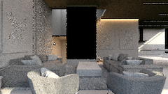
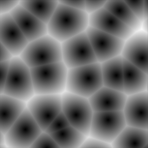
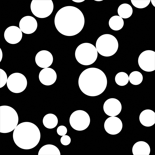
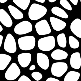
Blender has a Voronoi node
that can be used in any node based scenario (materials, compositor, geometry nodes). More precisely, it is
actually a Worley noise procedural noise function. It can be used
to produce various interesting patterns:

A typical implementation of Voronoi uses a hash function to randomly offset each grid cell. For something
like a 3D noise case, it has to calculate said hash on 27 neighboring cells (3x3x3), for each item
being evaluated. That is a lot of hashing!
Current implementation of e.g. “calculate random 0..1 3D offset for a 3D cell coordinate” looked like this in Blender:
// Jenkins Lookup3 Hash Function
// https://burtleburtle.net/bob/c/lookup3.c
#define rot(x, k) (((x) << (k)) | ((x) >> (32 - (k))))
#define mix(a, b, c) { \
    a -= c; a ^= rot(c, 4); c += b; \
    b -= a; b ^= rot(a, 6); a += c; \
    c -= b; c ^= rot(b, 8); b += a; \
    a -= c; a ^= rot(c, 16); c += b; \
    b -= a; b ^= rot(a, 19); a += c; \
    c -= b; c ^= rot(b, 4); b += a; \
}
#define final(a, b, c) { \
    c ^= b; c -= rot(b, 14); \
    a ^= c; a -= rot(c, 11); \
    b ^= a; b -= rot(a, 25); \
    c ^= b; c -= rot(b, 16); \
    a ^= c; a -= rot(c, 4); \
    b ^= a; b -= rot(a, 14); \
    c ^= b; c -= rot(b, 24); \
}
uint hash_uint3(uint kx, uint ky, uint kz)
{
    uint a;
    uint b;
    uint c;
    a = b = c = 0xdeadbeef + (3 << 2) + 13;
    c += kz;
    b += ky;
    a += kx;
    final(a, b, c);
    return c;
}
uint hash_uint4(uint kx, uint ky, uint kz, uint kw)
{
    uint a;
    uint b;
    uint c;
    a = b = c = 0xdeadbeef + (4 << 2) + 13;
    a += kx;
    b += ky;
    c += kz;
    mix(a, b, c);
    a += kw;
    final(a, b, c);
    return c;
}

float uint_to_float_incl(uint n)
{
    return (float)n * (1.0f / (float)0xFFFFFFFFu);
}
float hash_uint3_to_float(uint kx, uint ky, uint kz)
{
    return uint_to_float_incl(hash_uint3(kx, ky, kz));
}
float hash_uint4_to_float(uint kx, uint ky, uint kz, uint kw)
{
    return uint_to_float_incl(hash_uint4(kx, ky, kz, kw));
}
float hash_float3_to_float(float3 k)
{
    return hash_uint3_to_float(as_uint(k.x), as_uint(k.y), as_uint(k.z));
}
float hash_float4_to_float(float4 k)
{
    return hash_uint4_to_float(as_uint(k.x), as_uint(k.y), as_uint(k.z), as_uint(k.w));
}

float3 hash_float3_to_float3(float3 k)
{
    return float3(hash_float3_to_float(k),
        hash_float4_to_float(float4(k.x, k.y, k.z, 1.0)),
        hash_float4_to_float(float4(k.x, k.y, k.z, 2.0)));
}
i.e. it is based on Bob Jenkins’ “lookup3” hash function,
and does that “kind of three times”, pretending to hash float3(x,y,z), float4(x,y,z,1) and float4(x,y,z,2).
This is to calculate one offset of the grid cell. Repeat that to 27 grid cells for 3D Voronoi case.
I know! Let’s switch to PCG3D hash!
If you are aware of “Hash Functions for GPU Rendering” (Jarzynski, Olano, 2020) paper, you can
say “hey, maybe instead of using hash function from 1997, let’s use a dedicated 3D->3D hash function from several decades later”.
And you would be absolutely right:
uint3 hash_pcg3d(uint3 v)
{
  v = v * 1664525u + 1013904223u;
  v.x += v.y * v.z;
  v.y += v.z * v.x;
  v.z += v.x * v.y;
  v = v ^ (v >> 16);
  v.x += v.y * v.z;
  v.y += v.z * v.x;
  v.z += v.x * v.y;
  return v;
}
float3 hash_float3_to_float3(float3 k)
{
  uint3 uk = as_uint3(k);
  uint3 h = hash_pcg3d(uk);
  float3 f = float3(h);
  return f * (1.0f / (float)0xFFFFFFFFu);
}
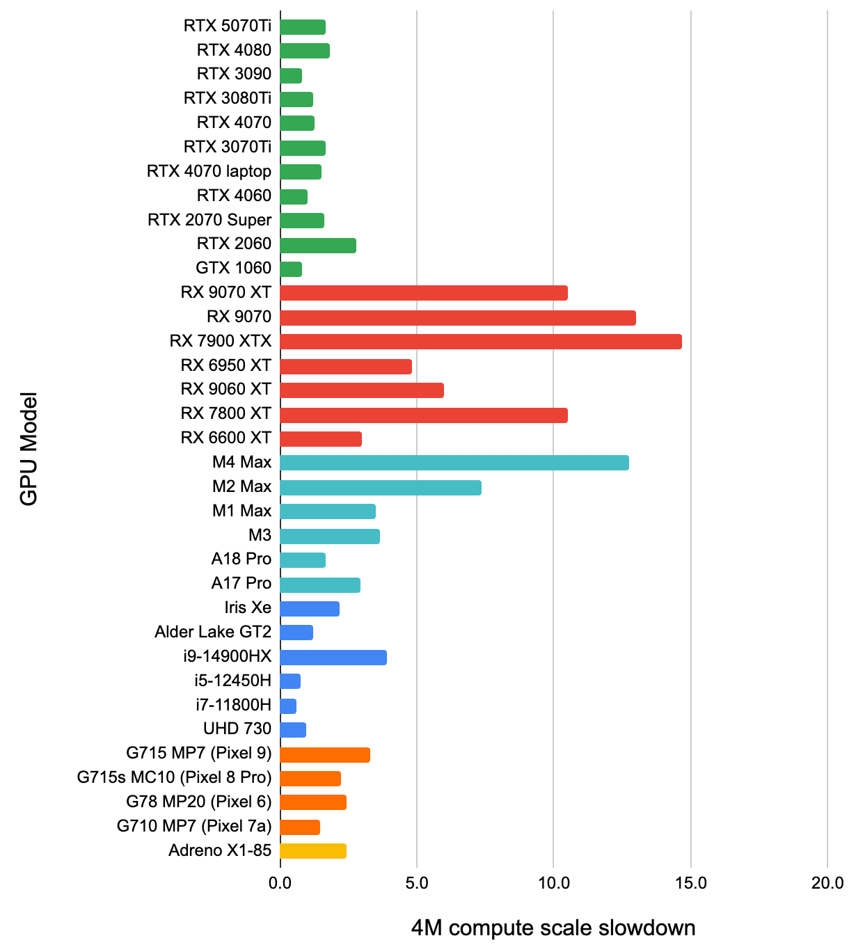
Which is way cheaper (the hash function itself is like 4x faster on modern CPUs). Good! We are done!
If you are using hash functions from the 1990s, try some of the more modern ones!
They might be both simpler and the same or better quality.
Hash functions from several decades ago were built on assumption
that multiplication is very expensive, which is very much not
the case anymore.
So you do this for various Voronoi cases of 2D->2D, 3D->3D, 4D->4D. First in the Cycles C++ code
(which compiles itself to both CPU execution, and to GPU via CUDA/Metal/HIP/oneAPI), then
in EEVEE GPU shader code (GLSL), then in regular Blender C++ code (which is used in geometry nodes
and CPU compositor).
And you think you are done until you realize…
Cycles with Open Shading Language (OSL)
The test suite reminds you that Blender Cycles can use OSL
as the shading backend. Open Shading Language, similar to
GLSL, HLSL or RSL, is a C-like language to write shaders in. Unlike some other languages, a “shader” does not output color;
instead it outputs a “radiance closure” so that the result can be importance-sampled by the renderer, etc.
So I thought, okay, instead of updating the Voronoi code in three places (Cycles CPU, EEVEE GPU, Blender CPU), it will have to
be four places. Let’s find out where and how does Cycles implements the shader nodes for OSL, update that place, and we’re good.
Except… turns out, OSL does not have unsigned integers (see data types).
Also, it does not have bitcast from float to int.
I certainly did not expect an “Advanced shading language for production GI renderers” to not have a concept of unsigned integers,
in year 2025 LOL :) I knew nothing about OSL just a day before, and now I was there wondering about the language data type system.
Luckily enough, specifically for Voronoi case, all of that can be worked around by:
- Noticing that everywhere within Voronoi code, we need to calculate a pseudorandom “cell offset” out of integer cell
coordinates only. That is, we do not need
hash_float3_to_float3, we need hash_int3_to_float3. This works around the lack
of bit casts in OSL.
- We can work around lack of unsigned integers with a slight modification to PCG hash, that just operates on signed integers instead.
OSL can do multiplications, XORs and bit shifts, just only on signed integers. Fine with us!
int3 hash_pcg3d_i(int3 v)
{
  v = v * 1664525 + 1013904223;
  v.x += v.y * v.z;
  v.y += v.z * v.x;
  v.z += v.x * v.y;
  v = v ^ (v >> 16);
  v.x += v.y * v.z;
  v.y += v.z * v.x;
  v.z += v.x * v.y;
  return v & 0x7FFFFFFF;
}
float3 hash_int3_to_float3(int3 k)
{
  int3 h = hash_pcg3d_i(k);
  float3 f = float3((float)h.x, (float)h.y, (float)h.z);
  return f * (1.0f / (float)0x7FFFFFFFu);
}
So that works, just instead of only having to change hash_float3_to_float3 and friends, this now required updating
all the Voronoi code itself as well, to make it hash integer cell coordinates as inputs.
“Wait, but how did Voronoi OSL code work in Blender previously?!”
Good question! It was using the OSL built-in hashnoise() functions
that take float as input, and produce a float output. And… yup, they just happened to use exactly the same Jenkins Lookup3 hash function underneath.
Happy coincidence? One implementation copying what the other was doing? I don’t know.
It would be nice if OSL got unsigned integers and bitcasts though. Since today, if you need to hash float->float, you can only use the built-in OSL
hash function, which is not particularly fast. For Voronoi case that can be worked around, but I bet there are other cases where workign around it is much harder.
So that’s it!
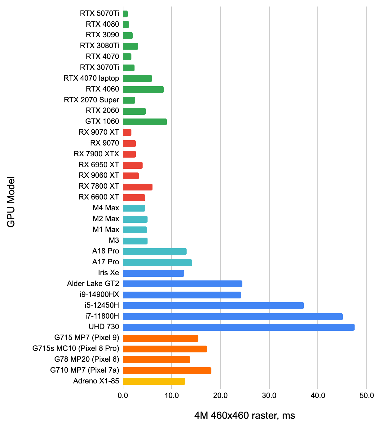
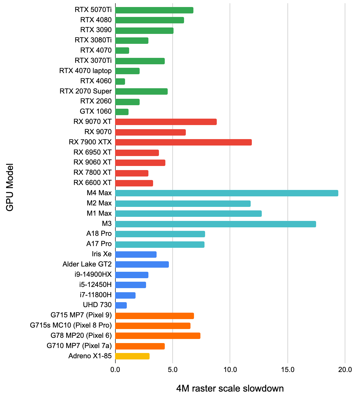
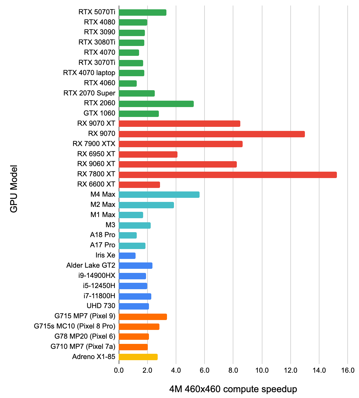
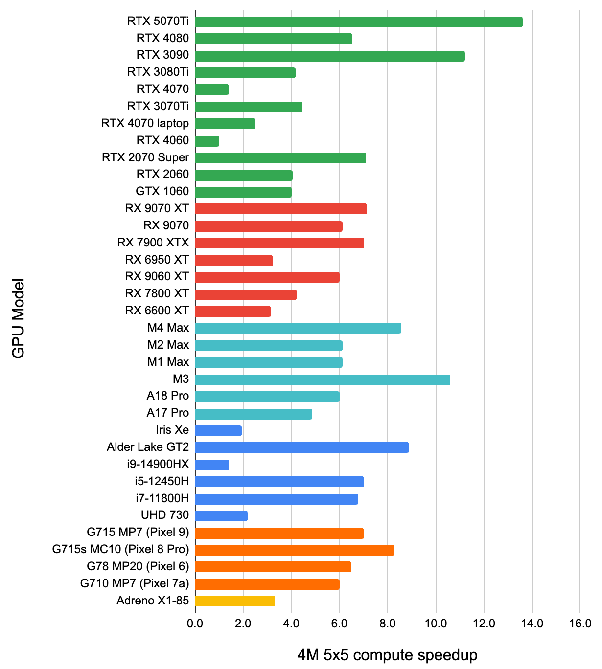
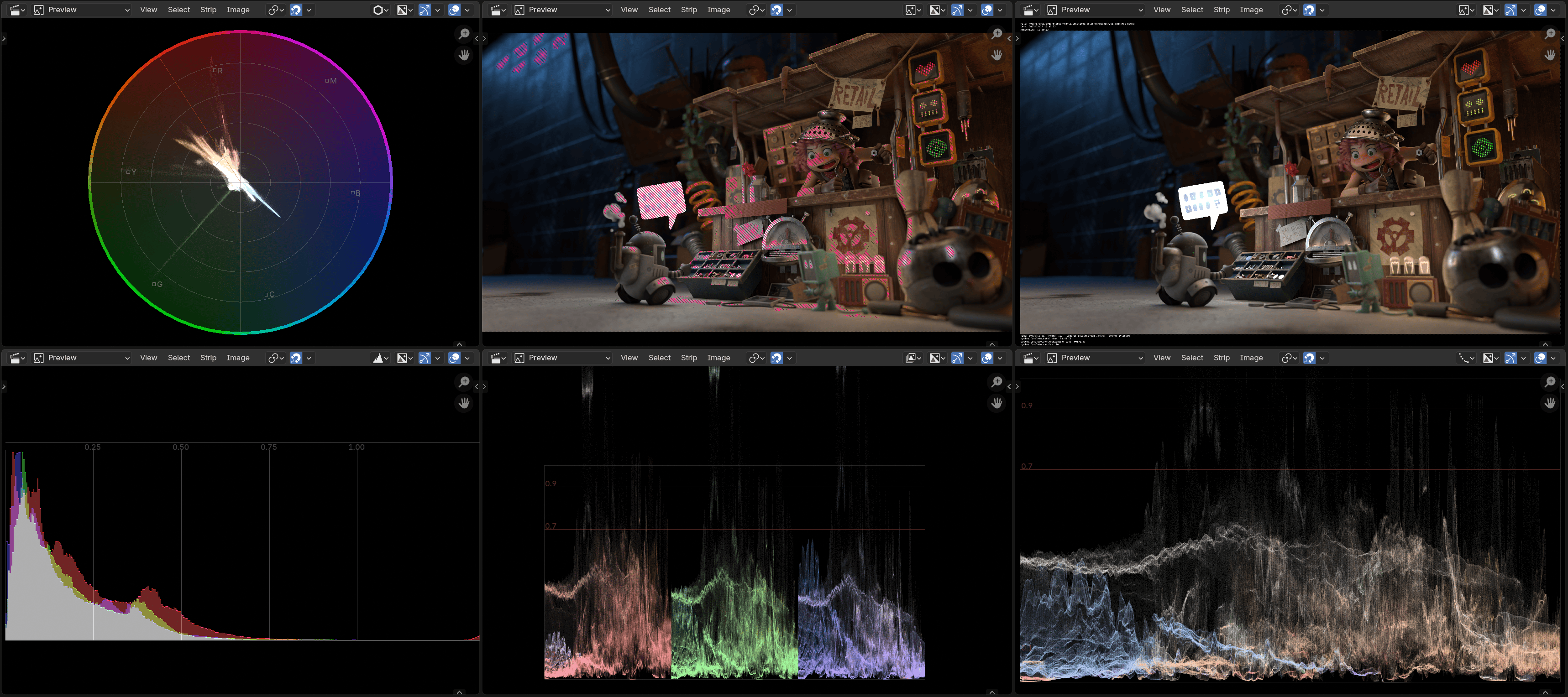
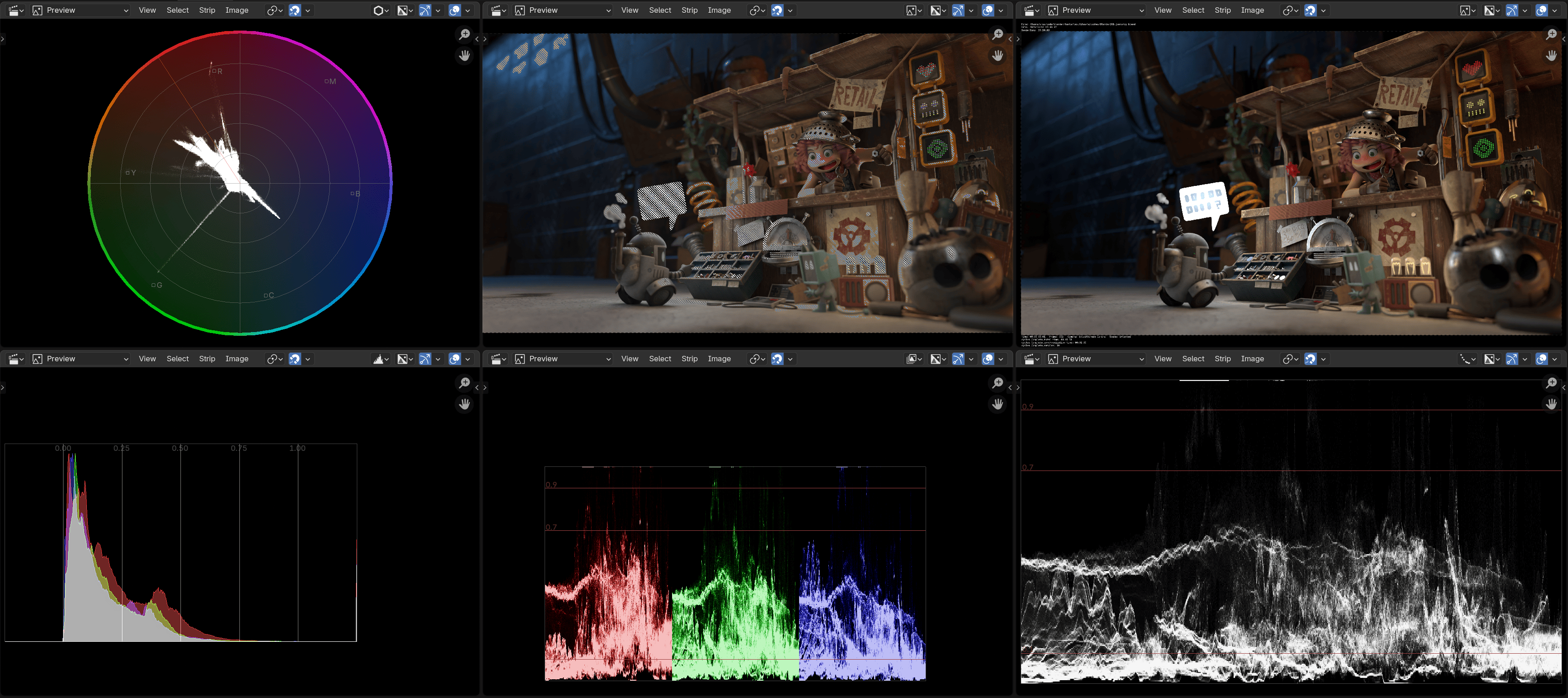
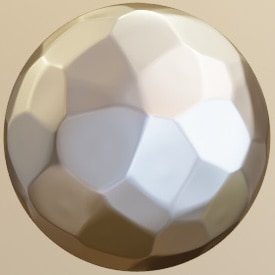
The pull request that makes Blender Voronoi node 2x-3x faster has been merged for Blender 5.0.
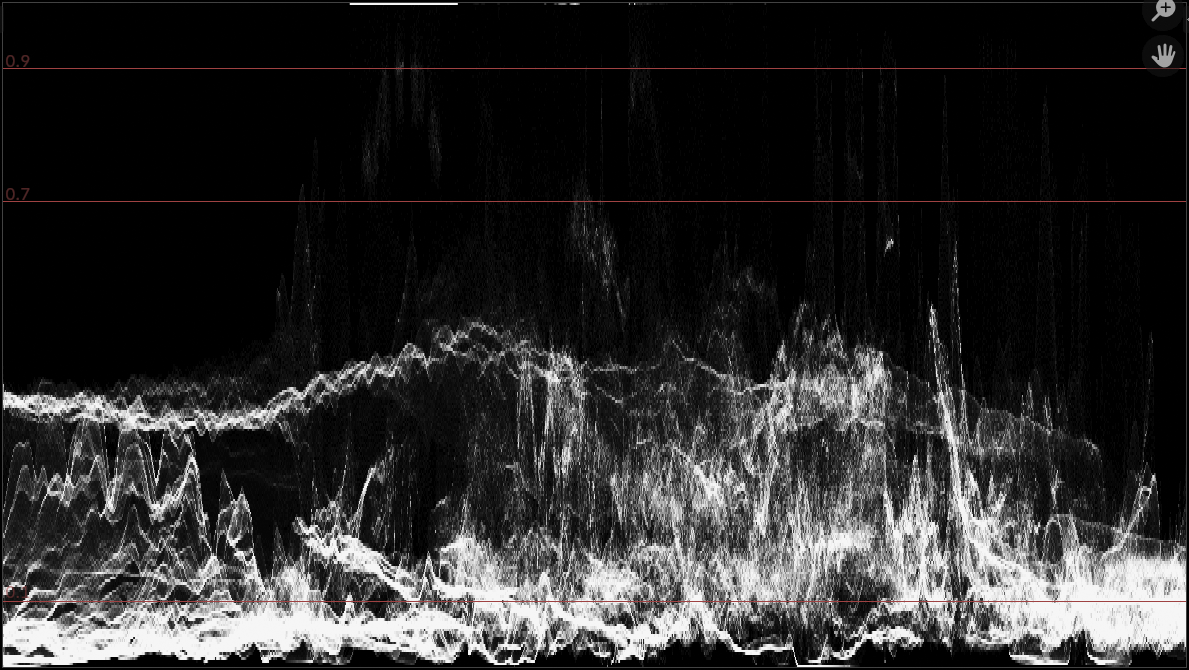
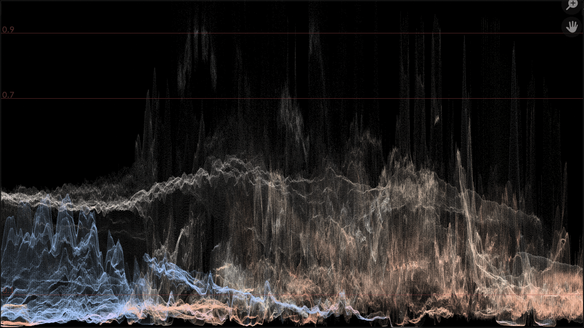
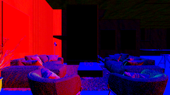
It does change the actual resulting Voronoi pattern, e.g. before and after:
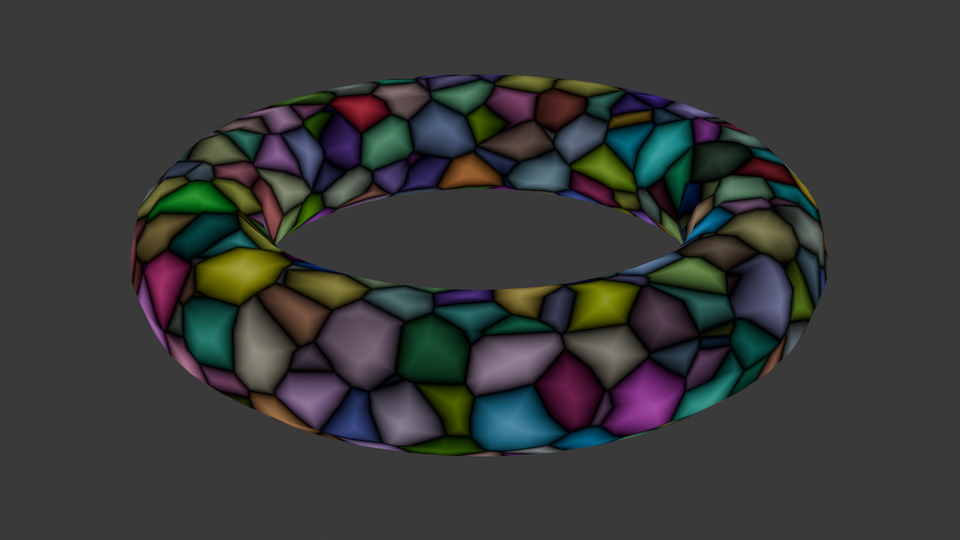
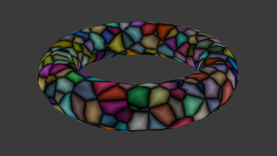
So while it “behaves” the same, the literal pattern has changed. And that is why a 5.0 release sounds like good timing to do it.
What did I learn?
- Actually learned about how Voronoi/Worley noise code works, instead of only casually hearing about it.
- Learned that various nodes within Blender have four separate implementations, that all have to match in behavior.
- Learned that there is a shading language, in 2025, that does not have unsigned integers :)
- There can be (and is) code out there that is using hash functions from the previous millenium, which might be not optimal today.
- I should still look at the SIMD aspect of this whole thing.
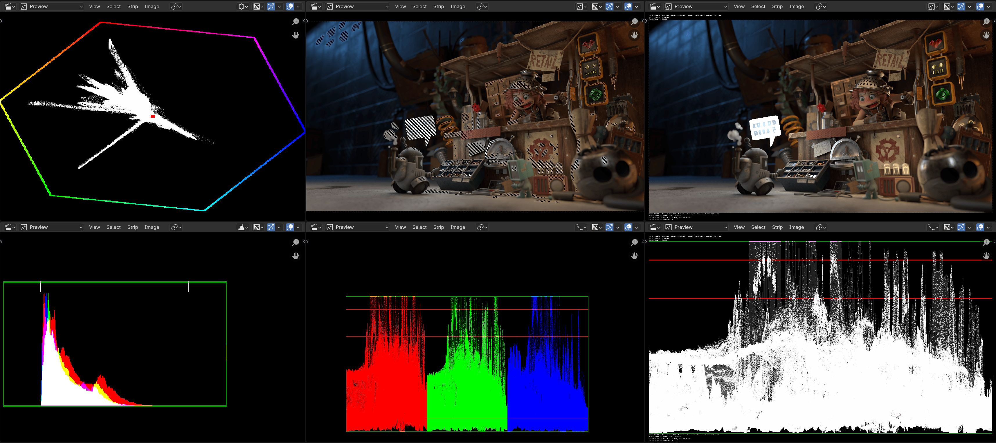
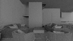
 Current Blender Studio production,